DRAFT: Stability-based evaluation of clusters using Seurat • countsplit.tutorials

We start by loading the necessary packages and installing the pbmc data. Note that this is the dataset used in the Seurat clustering tutorial, but is also included in the countsplit.tutorials package for convenience.

# Packages 
library(Seurat)
library(countsplit)
library(Matrix)
library(tidyverse)
library(patchwork)
library(sctransform)

# Load data and replace underscores with dashes in rownames (needed for Seurat)
data(pbmc.counts, package="countsplit.tutorials")
rownames(pbmc.counts) <- gsub(x = rownames(pbmc.counts), pattern = "_", replacement = "-")

Motivation

After preprocessing, the Seurat clustering tutorial applies Louvain clustering (as implemented in Seurat::FindClusters) to identify cell types in the data. The Louvain clustering algorithm has a resolution parameter that determines the granularity of the clustering, with larger values leading to greater numbers of clusters. The Seurat tutorial suggests that values between 0.4-1.2 typically return good results for single-cell datasets of around 3,000 cells (the size of the pbmc) dataset, but they note that this optimal value can increase for larger datasets. In the tutorial itself, they use 0.5 as the resolution parameter.

In this tutorial, our goal is to use count splitting to empirically determine an appropriate resolution parameter.

Let’s start by looking at the clusters originally estimated in the Seurat tutorial.

set.seed(1)
pbmc <- CreateSeuratObject(counts = pbmc.counts, min.cells = 5, min.features = 200)
pbmc <-
  pbmc %>%
  NormalizeData(verbose=F)  %>%
  FindVariableFeatures(verbose=F)  %>%
  ScaleData(verbose=F)  %>%
  RunPCA(verbose=F)  %>%
  FindNeighbors(dims = 1:10,verbose=F)  %>%
  RunUMAP(dims = 1:10,verbose=F) %>%
  FindClusters(resolution=0.5, verbose=F)
DimPlot(pbmc, reduction = "umap")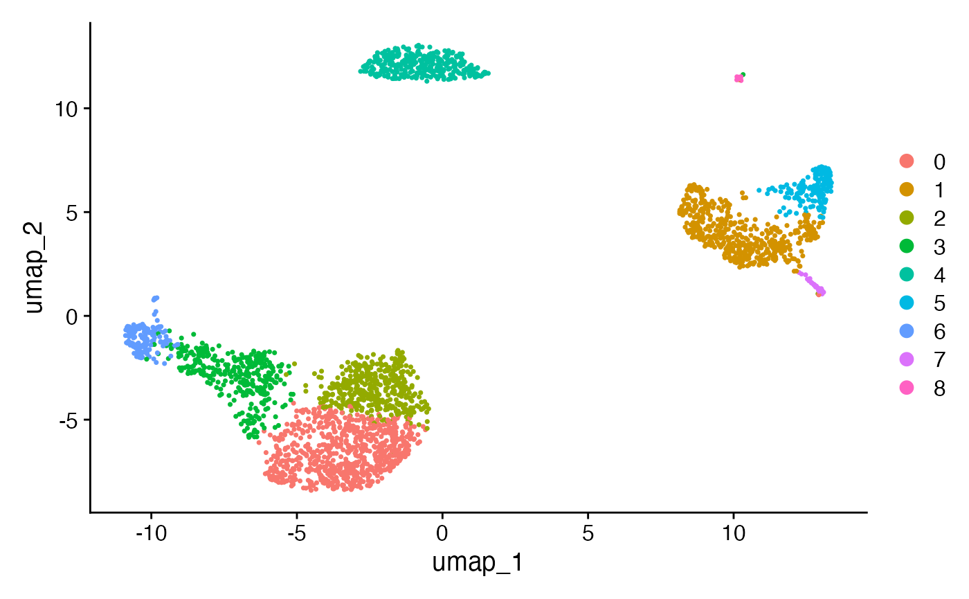

While the UMAP reduction has identified three clearly separated groups of cells, it is harder to tell if the subgroups of cells within the larger clusters are necessary. For example, what happens if make the same plot, but with a resolution parameter of 0.1 or 1.0?

pbmc <-
  pbmc %>%
  FindClusters(resolution=0.1, verbose=F) %>%
  FindClusters(resolution=1.0, verbose=F)
DimPlot(pbmc, reduction = "umap", group.by = paste0("RNA_snn_res.", c(0.1,1.0)))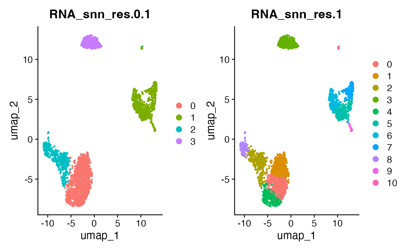

Based on this plot, there is no clear reason to think that the resolution parameter of 0.5 is better or worse than 0.1 or 1.0. In the remainder of this tutorial, we will show how count splitting can help us choose a resolution parameter.

Using count splitting

In our introduction to cluster evaluation tutorial, we used count splitting to choose the optimal number of clusters in a toy dataset. More specifically, we used the following workflow.

Use countsplit to turn a single dataset \(X\) into a training set \(X^{\mathrm{train}}\) and a test set \(X^{\mathrm{test}}\).
Estimate clusters using \(X^{\mathrm{train}}\).
Compute the within-cluster mean-squared-error (or a similar loss function) when the centers of these training-set clusters are used to predict the expression levels in \(X^{\mathrm{test}}\).

This represents a “reconstruction-based” evaluation of clusters. We want to know if the estimated cluster centers can get close to summarizing all of the information in our entire dataset. While this makes sense on toy datasets, it can get very complicated for real scRNA-seq data. For starters, we do not necessarily expect that our cell types will do a good job summarizing all of the variation in our sequencing data; they are just one important piece of the puzzle. Furthermore, it is not clear what loss function should be used in Step 3. Using the standard Seurat workflow, the clusters are estimated not on the raw counts but rather on the logged and size-factor-normalized counts, using only the features that were determined to be “highly variable”. Whether the loss function is computed using all of the features or only the highly variable features, for example, can really impact the results. Finally, this mean-squared-error is not particularly interpretable: how do we know what is a mean squared error that is “good” vs. “bad”?

For all of these complicated reasons, in this tutorial we take a different approach to evaluating our clusters. More specifically, we take a “reproducibility-based” approach. The basic premise is that, if we split our dataset \(X\) into independent \(X^{\mathrm{train}}\) and \(X^{\mathrm{test}}\), we want the clusters estimated on \(X^{\mathrm{train}}\) to be reproducible on \(X^{\mathrm{test}}\). The ``best” number of clusters for an analysis is the maximum number of clusters that achieves a specified threshold of reproducibility. This approach is similar to existing validation procedures based on cluster stability (Lange et al. (2004)) or “prediction strength” (Tibshirani and Walther (2005)).

Previous implementations of stability-based cluster evaluation have relied on repeated subsampling of the observations in the dataset. Stability can then only be assessed on observations that overlapped between the multiple subsamples. The nice thing about count splitting is that it lets us repeatedly cluster the exact same set of cells. This makes it a natural fit for these metrics.

We also briefly note that scRNA-seq cell types are not typically well-separated clusters, and sometimes truly are nested as main cell types and cell subtypes. This makes this problem really hard. In this document, we do not provide a perfect solution for the problem of estimating the number of clusters. But we do try to provide advice on how you might go about choosing the correct number of clusters in a principled way.

Poisson count splitting

We first demonstrate the idea using Poisson count splitting. At the bottom of the document, we repeat the same process but with negative binomial count splitting.

The first step is splitting the data into two identically distributed folds. Note that we set min.cells and min.features to \(0\) to turn off any automatic filtering. We want the rows and columns of the training set and the testing set to be identical, so we cannot filter them separately.

poissonSplit <- countsplit(t(pbmc.counts))
Xtrain <- t(poissonSplit[[1]])
Xtest <- t(poissonSplit[[2]])
pbmcTrain <- CreateSeuratObject(counts = Xtrain, min.cells = 0, min.features = 0)
pbmcTest <- CreateSeuratObject(counts=Xtest, min.cells=0, min.features=0)

The next step is to perform our preferred normalization pipeline on each dataset separately. Note that we filter both datasets to include the same rows and columns as the full dataset from above. This gets rid of genes and cells that had very little total expression.

pbmcTrain <-
  pbmcTrain[rownames(pbmc), colnames(pbmc)]  %>%
  NormalizeData(verbose=F) %>%
  FindVariableFeatures(verbose=F) %>%
  ScaleData(verbose=F) %>%
  RunPCA(verbose=F) %>%
  FindNeighbors(dims = 1:10, verbose=F) %>%
  RunUMAP(dims = 1:10, verbose=F)

pbmcTest <- pbmcTest[rownames(pbmc), colnames(pbmc)] %>%
  NormalizeData(verbose=F) %>%
  FindVariableFeatures(verbose=F) %>%
  ScaleData(verbose=F) %>%
  RunPCA(verbose=F) %>%
  FindNeighbors(dims = 1:10, verbose=F) %>%
  RunUMAP(dims = 1:10, verbose=F)

Now consider what happens if we cluster each dataset separately using a resolution parameter of 0.1, verses with a resolution parameter of 2.0.

pbmcTrain <-
  pbmcTrain %>%
  FindClusters(resolution=0.1, verbose=F) %>%
  FindClusters(resolution=2.0, verbose=F)
pbmcTest <-
  pbmcTest %>%
  FindClusters(resolution=0.1, verbose=F) %>%
  FindClusters(resolution=2.0, verbose=F)

Note that the results of each clustering got stored in the metadata of the relevant object, with the name RNA_snn_res.0.1 and RNA_snn_res.2. This is useful for us.

head(pbmcTrain@meta.data)

##                     orig.ident nCount_RNA nFeature_RNA RNA_snn_res.0.1
## AAACATACAACCAC-1 SeuratProject       1192          482               0
## AAACATTGAGCTAC-1 SeuratProject       2471          830               3
## AAACATTGATCAGC-1 SeuratProject       1554          693               0
## AAACCGTGCTTCCG-1 SeuratProject       1305          633               1
## AAACCGTGTATGCG-1 SeuratProject        490          303               2
## AAACGCACTGGTAC-1 SeuratProject       1089          492               0
##                  seurat_clusters RNA_snn_res.2
## AAACATACAACCAC-1               6             6
## AAACATTGAGCTAC-1               1             1
## AAACATTGATCAGC-1               0             0
## AAACCGTGCTTCCG-1              12            12
## AAACCGTGTATGCG-1              10            10
## AAACGCACTGGTAC-1               0             0

head(pbmcTest@meta.data)

##                     orig.ident nCount_RNA nFeature_RNA RNA_snn_res.0.1
## AAACATACAACCAC-1 SeuratProject       1227          471               0
## AAACATTGAGCTAC-1 SeuratProject       2430          808               3
## AAACATTGATCAGC-1 SeuratProject       1591          701               0
## AAACCGTGCTTCCG-1 SeuratProject       1332          580               1
## AAACCGTGTATGCG-1 SeuratProject        490          289               2
## AAACGCACTGGTAC-1 SeuratProject       1074          457               0
##                  seurat_clusters RNA_snn_res.2
## AAACATACAACCAC-1               9             9
## AAACATTGAGCTAC-1               0             0
## AAACATTGATCAGC-1               2             2
## AAACCGTGCTTCCG-1               6             6
## AAACCGTGTATGCG-1               8             8
## AAACGCACTGGTAC-1              10            10

I would like to visualize the two sets of clusterings in the same low-dimensional space. To do this, we will plot the cells in the training set UMAP space, colored with each potential clustering. To easily make this plot, we add the test set clusters to the training set meta data with the name testRNA_snn_res.

pbmcTrain@meta.data[["testRNA_snn_res.0.1"]] <- pbmcTest@meta.data[["RNA_snn_res.0.1"]]
pbmcTrain@meta.data[["testRNA_snn_res.2"]] <- pbmcTest@meta.data[["RNA_snn_res.2"]]

Now that the test set clusters are stored in the training set meta data, we can easily compare the following four plots.

DimPlot(pbmcTrain, reduction = "umap", group.by = c("RNA_snn_res.0.1", "testRNA_snn_res.0.1",
                                                    "RNA_snn_res.2", "testRNA_snn_res.2"))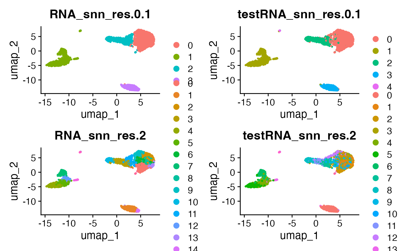

The takeaway from this plot is as follows. When we use a resolution parameter of 0.1, the clusters estimated on the training set are almost perfectly preserved on the test set. The only differences are that the tiny little cluster that is part of the green cluster in the training set becomes its own cluster in the test set, and that there is some fuzziness on the border of the blue/pink clusters. On the other hand, with a resolution parameter of 2, we can see that many of the clusters estimated on the training set are not preserved on the test set. This suggests that a parameter of 2 leads to too many clusters- because many are not reproducible.

If we estimate clusters for a wide range of resolution parameters, how do we quantify this degree of stability? One unfortunate issue with stability metrics is that the results are always the most stable with a small number of clusters; thus, the stability likely will not be minimized at the true number of clusters. However, we can come up with an interpretable metric for stability, and then select the largest number of clusters that achieves an acceptable threshold for this metric.

In this document, we use the metric from Tibshirani and Walther (2005). For every training set cluster, we compute the proportion of observation pairs in that cluster that are also assigned to the same cluster in the test set. We then take the minimum of this quantity over all training set clusters. The intuition is as follows. Suppose that there was some training set cluster where, in the test set, the observations got jumbled and all belonged to different clusters. Then this training set cluster probably should not have existed; i.e. there should have been at least one fewer cluster estimated on the training set. We implement this metric here:

stabilityLoss <- function(trainingClusters, testClusters) {
  uniqueTrain <- unique(trainingClusters) 
  minScore <- Inf
  for (clust in uniqueTrain) {
    obs1 <- which(trainingClusters==clust)
    testAssgt <- testClusters[obs1]
    total <- length(testAssgt) * (length(testAssgt) - 1)
    match <- sum(table(testAssgt) * (table(testAssgt) - 1)) 
    if (match/total < minScore) {
     minScore <- match/total
    }
  }
  return(minScore)
}

We note that many similar metrics could be proposed, but for now we stick with this one. Another option would be Jaccquard similarity, used in Tang et al. (2021).

We now cluster our training and test data for several resolution parameters and compute this metric.

resRange <- seq(0.1, 4, by = 0.1)
results.poisson <- rep(NA, length(resRange))

for (k in 1:length(resRange)) {
  pbmcTrain <- FindClusters(pbmcTrain, resolution = resRange[k], verbose=FALSE)
  pbmcTest <- FindClusters(pbmcTest, resolution = resRange[k], verbose=FALSE)
  
  ### The most recent clustering is always stored in "seurat_clusters". 
  clusters.train <-  pbmcTrain@meta.data[["seurat_clusters"]]
  clusters.test <-  pbmcTest@meta.data[["seurat_clusters"]]
  results.poisson[k] <- stabilityLoss(clusters.train, clusters.test)
}

We can now plot this metric. Recall that large values are preferable. We want to pick the largest value of the resolution parameter that achieves an acceptable value of this metric. Tibshirani and Walther (2005) suggested a cutoff of 0.8, but that was for well-separated clusters. As these clusters are not well-separated, we might be willing to go as low as 0.5.

ggplot(data=NULL, aes(x=resRange, y=results.poisson))+geom_point()+geom_line()+xlab("Resolution Parameter")+ylab("Stability of Clustering")+ggtitle("Poisson Count Splitting")+geom_hline(yintercept=0.5, col="red")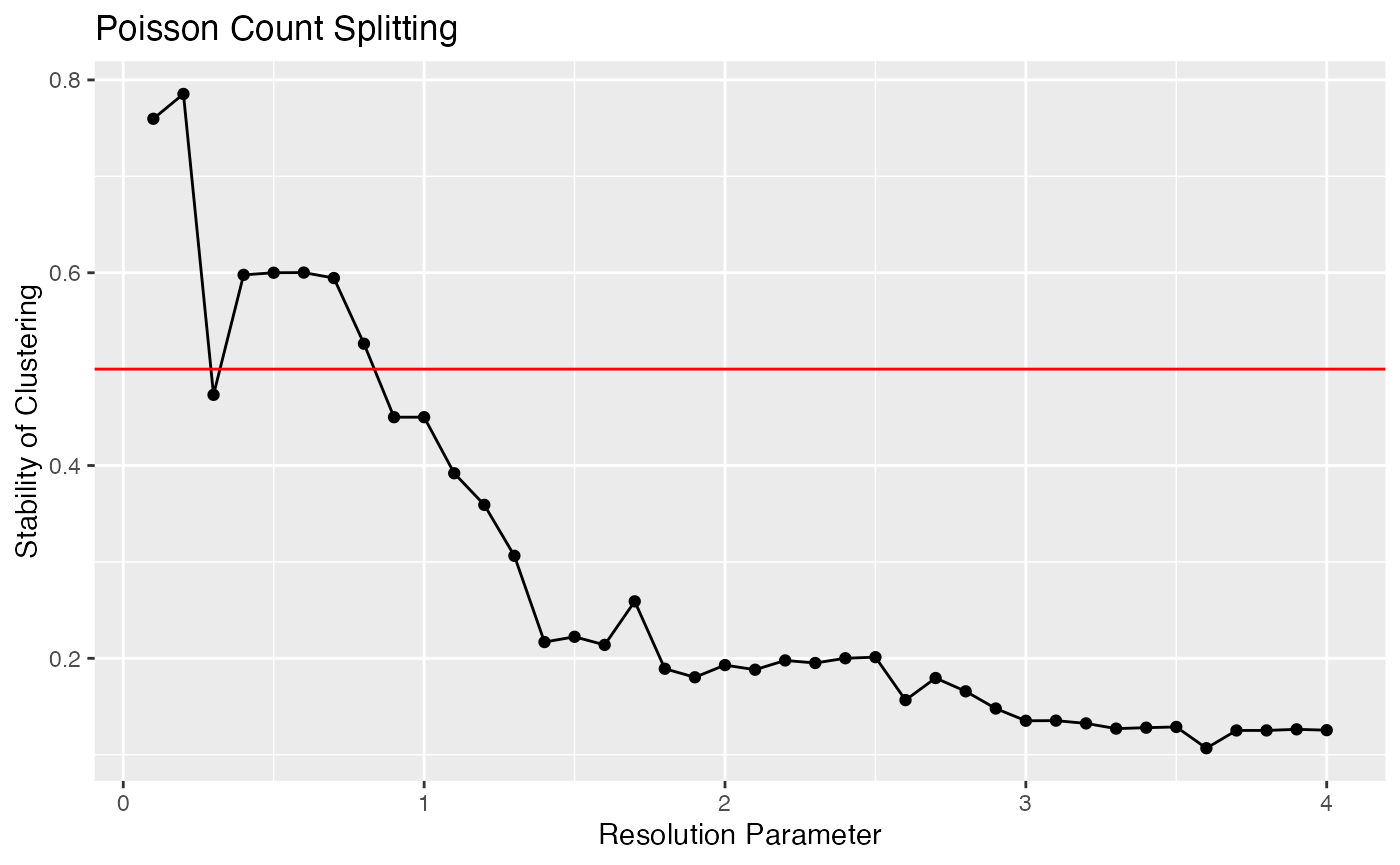

Based on this plot, when we use a resolution parameter of 0.7, the least reproducible cluster estimated on the training set is still 60% intact on the test set. For a resolution parameter of 1.5. that number drops to 20%. This is interpretable evidence that 1.5 is too large of a resolution parameter for this data, and that values larger than 0.7 or so should not be used.

Note that if we want to view UMAP plots of the training set or test set for any particular resolution parameter, we should do so as follows:

pbmcTrain@meta.data[[paste0("testRNA_snn_res.0.7")]] <- pbmcTest@meta.data[[paste0("RNA_snn_res.0.7")]]
DimPlot(pbmcTrain, reduction = "umap", group.by = c("RNA_snn_res.0.7", "testRNA_snn_res.0.7"))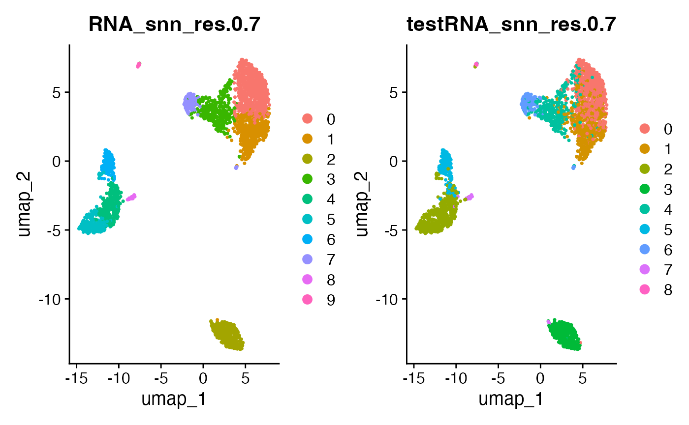

Note that, we could try repeating this procedure over multiple random splits to be even more sure of our findings. We do this below, for 15 random splits of the data.

nSplits <- 15
#resNames <- paste0("RNA_snn_res.", resRange)
results.poisson.multi <- matrix(NA, nrow=nSplits, ncol=length(resRange))

for (split in 1:nSplits) {
  poissonSplit <- countsplit(t(pbmc.counts))
  Xtrain <- t(poissonSplit[[1]])
  Xtest <- t(poissonSplit[[2]])
  pbmcTrain <- CreateSeuratObject(counts = Xtrain, min.cells = 0, min.features = 0)
  pbmcTest <- CreateSeuratObject(counts=Xtest, min.cells=0, min.features=0)

  pbmcTrain <-
    pbmcTrain[rownames(pbmc), colnames(pbmc)]  %>%
    NormalizeData(verbose=F) %>%
    FindVariableFeatures(verbose=F) %>%
    ScaleData(verbose=F) %>%
    RunPCA(verbose=F) %>%
    FindNeighbors(dims = 1:10, verbose=F) %>%
    RunUMAP(dims = 1:10, verbose=F)
  
  pbmcTest <- pbmcTest[rownames(pbmc), colnames(pbmc)] %>%
    NormalizeData(verbose=F) %>%
    FindVariableFeatures(verbose=F) %>%
    ScaleData(verbose=F) %>%
    RunPCA(verbose=F) %>%
    FindNeighbors(dims = 1:10, verbose=F) %>%
    RunUMAP(dims = 1:10, verbose=F)
  
  for (k in 1:length(resRange)) {
    pbmcTrain <- FindClusters(pbmcTrain, resolution = resRange[k], verbose=FALSE)
    pbmcTest <- FindClusters(pbmcTest, resolution = resRange[k], verbose=FALSE)
    
    ### This always stores the most recent run. 
    clusters.train <-  pbmcTrain@meta.data[["seurat_clusters"]]
    clusters.test <-  pbmcTest@meta.data[["seurat_clusters"]]
    results.poisson.multi[split, k] <- stabilityLoss(clusters.train, clusters.test)
  }
}

ggplot(data=NULL, aes(x=resRange, y=colMeans(results.poisson.multi)))+geom_point()+geom_line()+xlab("Resolution Parameter")+ylab("Average stability of clustering")+ggtitle("Multiple splits: Poisson")+
  geom_hline(yintercept=0.5, col="red")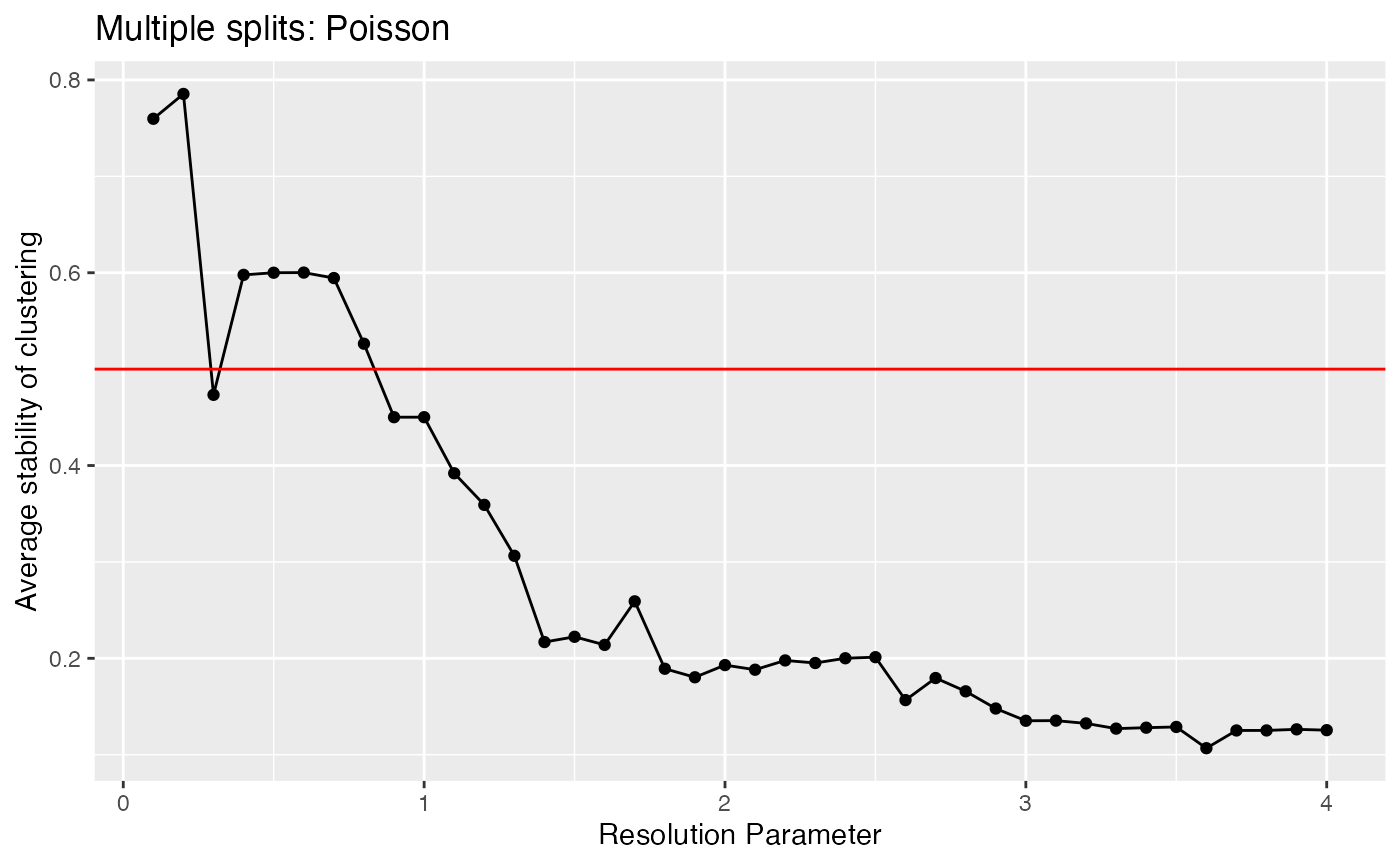

Negative binomial count splitting

It will be interesting to see if we get different results using negative binomial splitting. If anything, we should see less stability for a given resolution parameter, since with Poisson splitting we may have observed artificially high stability driven by correlation between the training set and the test set.

overdisps <- rep(Inf, nrow(pbmc.counts))
names(overdisps) <- rownames(pbmc.counts)
sctransform_fit <- sctransform::vst(pbmc.counts, verbosity=0, residual_type = "none", min_cells = 10, n_genes=5000)
overdisps[rownames(sctransform_fit$model_pars_fit)] <- sctransform_fit$model_pars_fit[,"theta"]

nbSplit <- countsplit(t(pbmc.counts))
Xtrain <- t(nbSplit[[1]])
Xtest <- t(nbSplit[[2]])
pbmcTrainNB <- CreateSeuratObject(counts = Xtrain, min.cells = 0, min.features = 0)
pbmcTestNB <- CreateSeuratObject(counts=Xtest, min.cells=0, min.features=0)

pbmcTrainNB <-
  pbmcTrainNB[rownames(pbmc), colnames(pbmc)]  %>%
  NormalizeData(verbose=F) %>%
  FindVariableFeatures(verbose=F) %>%
  ScaleData(verbose=F) %>%
  RunPCA(verbose=F) %>%
  FindNeighbors(dims = 1:10, verbose=F) %>%
  RunUMAP(dims = 1:10, verbose=F)

pbmcTestNB <- pbmcTestNB[rownames(pbmc), colnames(pbmc)] %>%
  NormalizeData(verbose=F) %>%
  FindVariableFeatures(verbose=F) %>%
  ScaleData(verbose=F) %>%
  RunPCA(verbose=F) %>%
  FindNeighbors(dims = 1:10, verbose=F) %>%
  RunUMAP(dims = 1:10, verbose=F)

results.nb <- rep(NA, length(resRange))

for (k in 1:length(resRange)) {
  pbmcTrain <- FindClusters(pbmcTrainNB, resolution = resRange[k], verbose=FALSE)
  pbmcTest <- FindClusters(pbmcTestNB, resolution = resRange[k], verbose=FALSE)
  
  ### The most recent clustering is always stored in "seurat_clusters". 
  clusters.train <-  pbmcTrain@meta.data[["seurat_clusters"]]
  clusters.test <-  pbmcTest@meta.data[["seurat_clusters"]]
  results.nb[k] <- stabilityLoss(clusters.train, clusters.test)
}


ggplot(data=NULL)+
  geom_line(aes(x=resRange, y=results.nb, col="Negative Binomial"))+
  geom_line(aes(x=resRange, y=results.poisson, col="Poisson"))+
  ylim(0,1)+ggtitle("Adding Negative Binomial Count Splitting")+xlab("Resolution Parameter")+ylab("Stability")+theme_bw()+geom_hline(yintercept=0.5, col="red")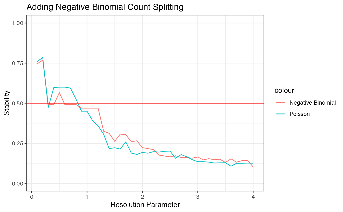

We can see that the curves produced by negative binomial count splitting and Poisson count splitting yield almost identical results here.

Summary

These stability metrics allow us to see that, if we choose a resolution parameter greater than 1, some of the clusters that we estimate are not reproducible. While this does not help us determine exactly the “correct” number of clusters, it is a fairly interpretable way to guide out choice. More work in this area is coming soon!

Citations

Lange, Tilman, Volker Roth, Mikio L Braun, and Joachim M Buhmann. 2004. “Stability-Based Validation of Clustering Solutions.” Neural Computation 16 (6): 1299–1323.

Tang, Ming, Yasin Kaymaz, Brandon L Logeman, Stephen Eichhorn, Zhengzheng S Liang, Catherine Dulac, and Timothy B Sackton. 2021. “Evaluating Single-Cell Cluster Stability Using the Jaccard Similarity Index.” Bioinformatics 37 (15): 2212–14.

Tibshirani, Robert, and Guenther Walther. 2005. “Cluster Validation by Prediction Strength.” Journal of Computational and Graphical Statistics 14 (3): 511–28.