Tutorial: countsplitting and scran

Before using this tutorial, we recommend that you read through our introductory tutorial to understand our method in a simple example with simulated data.

In this tutorial, we use a real dataset from Elorbany et al. (2022). The dataset contains 10,000 cells collected over 15 days of a directed differentiation protocol from induced pluripotent stem cells (IPSC) to cardiomyocytes (cm).

Overview

After loading the necessary software and performing count splitting, in this tutorial we carry out the following steps.

• Preprocessing: We preprocess the training data using the preprocessing steps suggested by the scran tutorial.

• Clustering: We cluster the cells using scran using the preprocessed training data.

• Differential Expression Analysis: Using the test data, we test to see which genes are associated with the estimated clusters. We do this both “by hand” using Poisson GLMs as well as using the built-in methods from the scran package.

Install scran

If you don’t already have scran, you will need to run:

if (!require("BiocManager", quietly = TRUE))
    install.packages("BiocManager")
BiocManager::install("scran")

Next, you should load the package, along with others that we will use in this tutorial.

library(scran)
library(tidyverse)
library(countsplit)
library(countsplit.tutorials)

Load the data and perform count splitting

This data is included in the countsplit_tutorials package as a SingleCellExperiment object, so it is simple to load.

data(cm)
cm

## class: SingleCellExperiment 
## dim: 21971 10000 
## metadata(0):
## assays(1): counts
## rownames(21971): AL627309.1 AL627309.6 ... AC136352.4 AC007325.4
## rowData names(0):
## colnames(10000): E1_E1CD3col4_CATTTGTGCTTG E1_E1CD3col2_AGAATAAGTCAC
##   ... E1_E1CD1col5_GTTACGCTAGTG E1_E1CD2col4_CCGCACAAGATC
## colData names(26): orig.ident nCount_RNA ... pseudotime ident
## reducedDimNames(0):
## mainExpName: NULL
## altExpNames(0):

The main item in cm that we care about is the counts matrix, which contains 21,971 genes and 10000 cells. We can view a small subset of it now.

dim(counts(cm))
## [1] 21971 10000
counts(cm)[1:10,1:10]
## 10 x 10 sparse Matrix of class "dgCMatrix"
##   [[ suppressing 10 column names 'E1_E1CD3col4_CATTTGTGCTTG', 'E1_E1CD3col2_AGAATAAGTCAC', 'E2_E2CD2col5_ATGAATGATGAA' ... ]]
##                                 
## AL627309.1  .  . . . . . . . . .
## AL627309.6  .  . . . . . . . . .
## AL627309.5  .  . . . . . . . . .
## AL669831.3  .  . . . . . . . . .
## MTND1P23    1 12 . . 3 1 . . 4 .
## MTND2P28    6  3 . . . . 2 1 . .
## MTCO1P12    2  7 2 . 2 . 1 2 3 .
## MTCO2P12    .  1 . . . . . . . .
## MTATP8P1    .  . . . . . . . . .
## MTATP6P1   10  8 . . . . 3 . 2 .

There is other important information included in the cm object. For example, the cells were collected from 19 individuals over the course of 15 days. Information on which individual and which day each cell is from is saved within the cm object as column data.

table(cm$individual)
## 
## 18520 18912 19093 18858 18508 18511 18907 18505 19190 18855 19159 18489 18517 
##   472   760   925   732   581   701   362   438   524   283   326   400   534 
## 18499 18870 19193 19209 19108 19127 
##   771   700   373   554   211   353
table(cm$diffday)
## 
##  day0  day1  day3  day5  day7 day11 day15 
##  2383  2389  1691   967  1260   862   448

To perform Poisson count splitting we wish to extract only the count matrix.

set.seed(1)
X <- counts(cm)
split <- countsplit(X)

## As no overdispersion parameters were provided, Poisson count splitting will be performed.

Xtrain <- split[[1]]
Xtest <- split[[2]]

Preprocess the training set.

We now wish to compute clusters on the training set. Unlike in our introductory tuorial, instead of simply running kmeans() on log(Xtrain+1), we will use an existing scRNA-seq pipeline from the scran package that also involves preprocessing steps such as selecting highly variable genes. In order to do this, we need to store the training set count matrix Xtrain in a SingleCellExperiment object.

We could make a new SingleCellExperiment object that contains only the Xtrain counts matrix. However, this would discard all of the metadata that was stored in the cm object, such as information regarding which cells where collected on which days and from which individuals. Thus, we chose to let cm.train be a copy of cm where we only update the counts() attribute. This way, all metadata from cm is retained in cm.train.

cm.train <- cm
counts(cm.train) <- Xtrain

Now we are ready for our analysis. These steps were inspired by the scran tutorial. We first compute sum factors and then we perform log normalization. Note that the computeSumFactors() function requires computing initial clusters of cells using quickCluster(); these are different from the clusters of cells that we will later analyze for differential expression.

clusters <- quickCluster(cm.train)
cm.train <- computeSumFactors(cm.train, clusters=clusters)
cm.train <- logNormCounts(cm.train)

We then compute the top 2000 highly variable genes. While this step does not alter the dimension of counts(cm.train), it allows us to later perform clustering or dimension reduction using only these highly variable genes.

top.hvgs <- getTopHVGs(modelGeneVar(cm.train), n=2000)

Finally, we perform dimension reduction on the dataset (using only the highly variable genes).

cm.train <- fixedPCA(cm.train, subset.row=top.hvgs)

Cluster the training set

We cluster the dimension-reduced dataset using scran’s clusterCells function (which performs graph-based clustering).

clusters.train <- clusterCells(cm.train,use.dimred="PCA")

It turns out that this function returned 11 clusters. We can visualize them below.

table(clusters.train)
ggplot(as_tibble(reducedDim(cm.train)), aes(x=PC1, y=PC2, col=as.factor(clusters.train)))+geom_point()+labs(col="Cluster")

## Don't know how to automatically pick scale for object of type
## <reduced.dim.matrix/matrix>. Defaulting to continuous.
## Don't know how to automatically pick scale for object of type
## <reduced.dim.matrix/matrix>. Defaulting to continuous.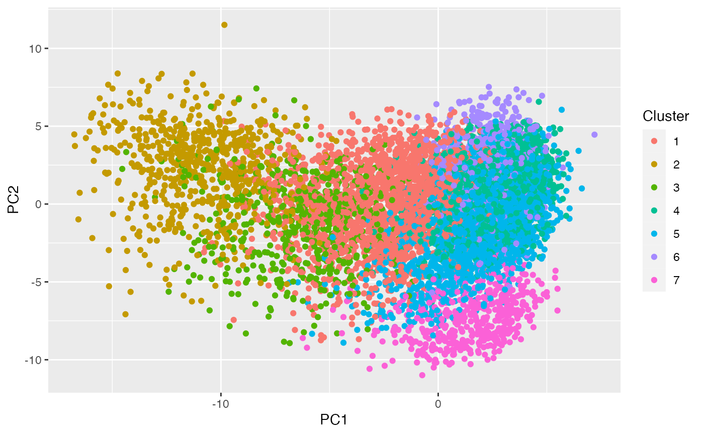

Differential expression testing

Using Poisson GLMs

We now consider fitting Poisson GLMs to test for differential expression between clusters 1 and 2. We can do this analysis “by hand”, meaning that we do not need to store Xtest in a SingleCellExperiment object.

For computational efficiency, we test 500 randomly selected genes for differential expression, rather than checking all 21,000 genes. The first step is to subset the test data to only include these 500 genes and to only include cells that were placed in cluster 1 or cluster 2. We will include size factors for each cell, estimated on the training set, as offsets in our Poisson GLM. We need to obtain the appropriate size factor vector and subset it to only include the cells that were placed in cluster 1 or cluster 2. We do these steps below.

set.seed(1)
indices <- which(clusters.train==1 | clusters.train==2)
genes <- sample(1:NCOL(Xtest), size=500) 
Xtestsubset <- Xtest[genes, indices]
sizefactors.subset <- sizeFactors(cm.train)[indices]

We are now ready to test for differential expression. We see that 61 out of our 500 genes were identified as significantly differentially expressed at alpha=0.01.

results <- t(apply(Xtestsubset, 1, function(u) summary(glm(u~clusters.train[indices], offset=log(sizefactors.subset), family="poisson"))$coefficients[2,]))
table(results[,4] < 0.01) 
## 
## FALSE  TRUE 
##   439    61

We can view the names of these highly significant genes below.

head(results[results[,4] < 0.01,], n=10)
##           Estimate Std. Error   z value     Pr(>|z|)
## C3orf62  1.2324039 0.43690137  2.820783 4.790661e-03
## PPFIA4   1.6967096 0.62676308  2.707099 6.787406e-03
## CDCA7L   0.6235322 0.14797067  4.213890 2.510091e-05
## ZFR      0.2439864 0.08567689  2.847750 4.402946e-03
## SELENOT  0.5564246 0.18215736  3.054637 2.253332e-03
## COL11A2  2.9288532 1.08012328  2.711592 6.696103e-03
## FAM241A  1.6967096 0.62676433  2.707093 6.787516e-03
## PPP2R5A  0.5493071 0.21081767  2.605603 9.171275e-03
## ZNF138  -0.8594601 0.32129460 -2.674991 7.473132e-03
## ZNF436   1.6070974 0.57008420  2.819053 4.816561e-03

Using scran

In this section, instead of testing for differential expression “by hand” using glm(), we use the scoreMarkers() function from the scran package. This is the method used in the scran tutorial, in the section titled “Find Marker Genes”.

In order to use the scoreMarkers() function, we need to store our test matrix in a SingleCellExperiment object. We can either construct this from scratch using only the count matrix, or we could make a copy of the original cm object and add the count matrix after. Since we do not anticipate needing any metadata in this section, we construct the object from scratch.

cm.test <- SingleCellExperiment(list(counts=Xtest))

The scoreMarkers() function needs access to the log-normalized counts assay (logcounts()) in the cm.test object. To fill in this assay, we need to run the logNormCounts function on cm.test. We would like to normalize the test matrix using size factors computed on the training set (this follows our general philosophy of performing all preprocessing steps on the training set). Thus, we obtain size factors from the training set before calling logNormCounts().

sizeFactors(cm.test) <- sizeFactors(cm.train)
cm.test <- logNormCounts(cm.test) 

This first element in results shows marker genes that distinguish cluster 1 from all other clusters.

results <- scran::findMarkers( 
cm.test, groups= clusters.train,
 pval.type = "all") 
results[[1]]

## DataFrame with 21971 rows and 9 columns
##               p.value         FDR summary.logFC     logFC.2     logFC.3
##             <numeric>   <numeric>     <numeric>   <numeric>   <numeric>
## TPM1      1.08718e-87 2.38865e-83      1.524155    -2.60820   -1.691339
## TNNT2     3.92556e-20 3.42042e-16      0.243453    -2.74309   -0.629304
## MYL7      4.67036e-20 3.42042e-16     -0.619474    -3.00084   -0.619474
## NEXN      6.38871e-17 3.50916e-13      0.180813    -1.26727   -0.599001
## ANKRD1    8.78375e-17 3.85975e-13      0.256620    -1.45896   -1.366888
## ...               ...         ...           ...         ...         ...
## GABRQ               1           1             0  0.00000000  0.00000000
## CLIC2               1           1             0  0.00000000 -0.00355741
## EEF1A1P41           1           1             0 -0.00491876  0.00000000
## PCDH11Y             1           1             0  0.00000000  0.00000000
## TMSB4Y              1           1             0  0.00000000  0.00000000
##                logFC.4      logFC.5      logFC.6     logFC.7
##              <numeric>    <numeric>    <numeric>   <numeric>
## TPM1          1.393705     1.539964     1.764288    1.524155
## TNNT2         0.261539     0.284571     0.299269    0.243453
## MYL7          0.511705     0.595673     0.518480    0.422453
## NEXN          0.165924     0.185703     0.184252    0.180813
## ANKRD1        0.300527     0.322272     0.295123    0.256620
## ...                ...          ...          ...         ...
## GABRQ     -0.004987919 -0.002776015  0.000000000  0.00000000
## CLIC2     -0.000899236  0.000000000 -0.002090804  0.00000000
## EEF1A1P41 -0.000239274  0.000000000  0.000000000  0.00000000
## PCDH11Y   -0.001452754 -0.001119289 -0.000813786  0.00000000
## TMSB4Y     0.000000000 -0.000292628  0.000000000 -0.00585973

Even with count splitting, we identify several highly significant marker genes, both “by hand” and with the findMarkers() function.

References

Elorbany, Reem, Joshua M Popp, Katherine Rhodes, Benjamin J Strober, Kenneth Barr, Guanghao Qi, Yoav Gilad, and Alexis Battle. 2022. “Single-Cell Sequencing Reveals Lineage-Specific Dynamic Genetic Regulation of Gene Expression During Human Cardiomyocyte Differentiation.” PLoS Genetics 18 (1): e1009666.